Lab 12: Path Planning and Execution

Full Bluetooth commanded mapping! Navigating through the room with local path planning.

Objective

The final lab objective is to command the robot to navigate through a set of checkpoints and map out the room with the ToF sensors and the Bayes Filter. This combines the mapping in Lab 9 and the localization in Lab 11, but with commanded movement between each checkpoint instead of manual.

I opted for open-loop control, combining the 360 degree orientation control with the previously-built Bluetooth drive commands, allowing the robot to drive forward or backwards, left or right for any speed and duration. With this method, I would have full control of the robot. Although this is slower compared to full closed-loop control and requires more monitoring, it allows me to correct the robot's path and ensure each checkpoint is reached.

I followed the recommended path in the Lab notes:

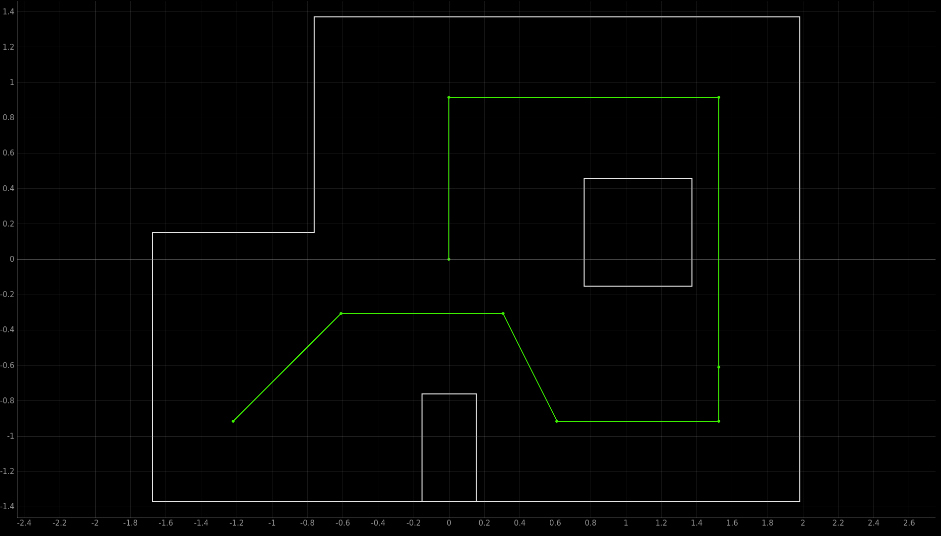
The procedure was:

• Initialize the beliefs and then run the update step of the Bayes Filter at the current point.
• If the output belief matches the expected location, store the ToF and locaation data in a CSV file. Otherwise, rerun the update step.
• Command open-loop control to the next checkpoint, starting at 0 degrees.
• Repeat for every checkpoint.

Sending, Receiving, and Saving Data

I first faced issues with the robot's memory, since the IMU, ToF, and Kalman Filter arrays would fill up the available memory and cause the robot to be stuck in its current state (ex. spinning forever). This was not a problem in previous labs since the trials would be under 1 minute. However, to have a continuous navigation trial, I needed to store only the necessary data.

Therefore, I decided that the ToF and Kalman Filter data would only be sent over Bluetooth, since only the values at each angle increment were needed. When each increment was reached, the latest distanceFront value was sent to the notification handler. I removed the send_increments function from Lab 11.

In the main loop:

    ...
        if (angleTraveled < 360){
          pwm = PID_angle_control();
          get_PWM();

          int pwm_max = 255 * Spa;
          int pwm_min = 110;
          abs_pwm = abs(pwm) * pwm_max / 100;

          if (abs(errorCur) < pwm_angle_tolerance) {
            driveState = STOP;
            Serial.println("next angle");

            tx_estring_value.clear();
            tx_estring_value.append("Sensor:");
            tx_estring_value.append(distanceFront);  
            tx_estring_value.append(";");

            tx_characteristic_string.writeValue(tx_estring_value.c_str());

            angleWanted += increment;
            angleTraveled += increment;
            Serial.println(angleTraveled);
          } else {

            if (abs_pwm > pwm_max) abs_pwm = pwm_max;
            if (abs_pwm < pwm_min) abs_pwm = pwm_min;

            if (pwm > 0.0) driveState = RIGHT;
            else if (pwm < 0.0) driveState = LEFT;
          }   
        } else {
            stop();
            driveState = STOP;
            collectPIDangle = 0;
            angleInitialized = 0;
            for (int i = 0; i < 2; i++) {
                digitalWrite(LED_BUILTIN, HIGH);
                delay(300);
                digitalWrite(LED_BUILTIN, LOW);
                delay(300);
            }
        }
    ...

Then, the notification handler appended the data to an array:

    def notification_handler(self, uuid, byte_array):
        msg = self.ble.bytearray_to_string(byte_array).strip()
    
        if msg.startswith("Sensor:"):
            try:
                parts = msg.split(";")
                val = np.float64(parts[0].split(":")[1])
                
                self.sensor_ranges.append(val/1000.0)

A save_data function was called at each checkpoint:

def save_data(filename, pose, sensor_ranges):
    file_exists = os.path.isfile(filename)
    ranges = sensor_ranges.flatten().tolist()

    row = [pose[0], pose[1], pose[2]] + ranges

    with open(filename, 'a', newline='') as f:
        writer = csv.writer(f)

        if not file_exists:
            header = ["x", "y", "theta"] + [f"Measurement {i+1}" for i in range(len(ranges))]
            writer.writerow(header)

        writer.writerow(row)

I manually determined if the data at each checkpoint was valid and saved it:

argmax_bel = get_max(loc.bel)
current_belief = mapper.from_map(*argmax_bel[0])

save_data(
    "Data.csv",
    current_belief,
    loc.obs_range_data
)

Python Mapping

The data were saved in CSV files, with each row containing the state belief, and the 18 ToF measurements. The data were read and plotted to show the state beliefs:

df = pd.read_csv("success2.csv")
M_TO_FT = 3.28084

df["x_ft"] = df["x"] * M_TO_FT
df["y_ft"] = df["y"] * M_TO_FT

plt.figure(figsize=(8,8))
plt.scatter(df["x_ft"], df["y_ft"], s=80)
for i, row in df.iterrows():
    plt.text(
        row["x_ft"],
        row["y_ft"],
        str(i + 1),
        fontsize=9
    )

arrow_len = 0.5  # ft
theta_rad = np.deg2rad(df["theta"])

u = arrow_len * np.cos(theta_rad)
v = arrow_len * np.sin(theta_rad)

plt.quiver(
    df["x_ft"],
    df["y_ft"],
    u,
    v,
    angles='xy',
    scale_units='xy',
    scale=1
)

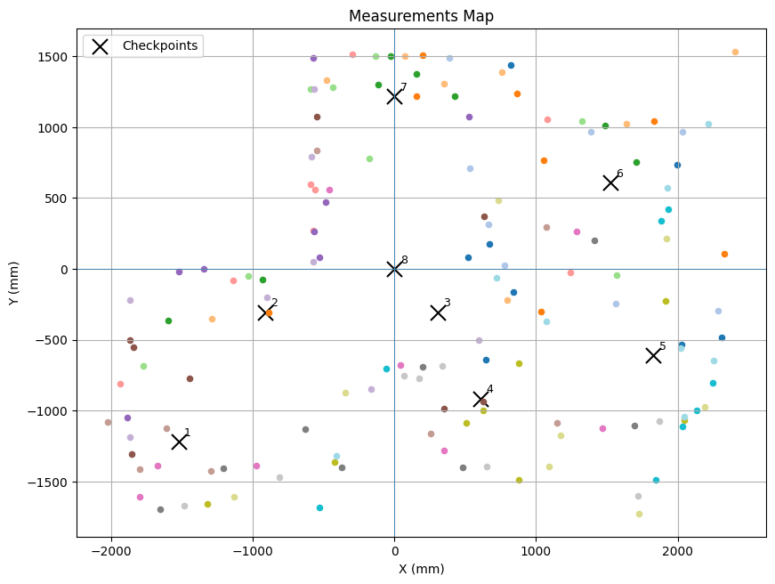
The ToF measurements were plotted onto a single graph. The polar coordinates were converted to cartesian. Additionally, the angleOffset and tofOffset values were manually evaluated based on the mapping results.

x0 = df["x"].values * 1000
y0 = df["y"].values * 1000

measurement_cols = df.columns[3:]

angles_deg = np.arange(0, len(measurement_cols) * 20, 20)

angles_rad = np.deg2rad(angles_deg + angle_offset)

plt.figure(figsize=(10, 8))

plt.scatter(
    x0,
    y0,
    s=150,
    color='black',
    marker='x',
    label='Checkpoints'
)

for i in range(len(df)):
    plt.text(
        x0[i] + 40,
        y0[i] + 40,
        str(i + 1),
        fontsize=9
    )

colors = plt.cm.tab20(np.linspace(0, 1, len(measurement_cols)))
tofOffset = 0
angleOffset = np.deg2rad(20)

for angle, col, color in zip(angles_rad, measurement_cols, colors):

    r = df[col].values * 1000

    xm = x0 + (r - tofOffset) * np.cos(angle + angleOffset)
    ym = y0 + (r - tofOffset) * np.sin(angle + angleOffset)

    plt.scatter(
        xm,
        ym,
        s=20,
        color=color,
    )

Trials

Multiple trials were tested at various minimum speeds.

Trial 1: Minimum PWM = 95

The full path trajectory is shown below (split into 3 video segments):

The Python command side was also recorded (note that the time is longer due to retrying multiple checkpoints):

Then, the resulting position and angle beliefs were printed, as well as the map generated from the ToF readings.

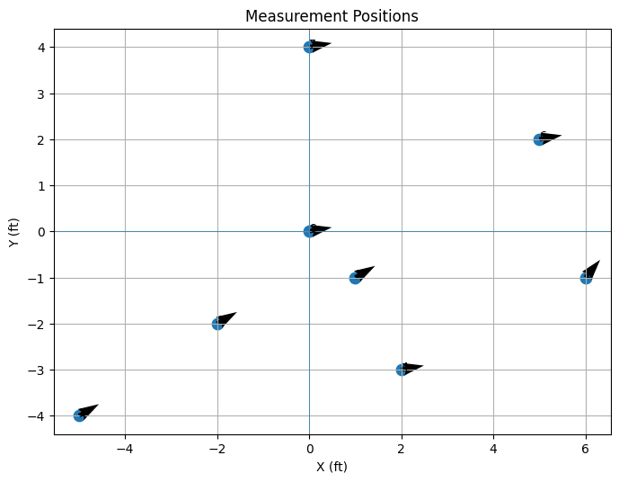
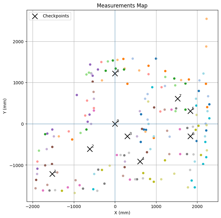
Trial 2: Minimum PWM = 110

I decided to increase the robot's minimum PWM to speed up the pathing process from the previous trial. The tradeoff in the improved speed was the ToF measurement accuracy.

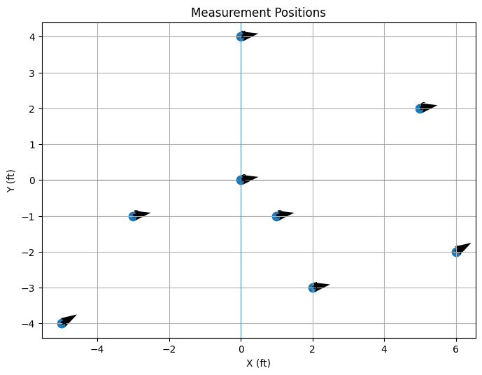
The final results were as follows:

Conclusions

Overall, Trial 2 resulted in a more accurate state measurement and a more reliable mapping compared to Trial 1. The increase in PWM actually allowed the turning to be more centered about the axis, since both set of wheels could overcome friction easily. The entire mapping sequence was ~9 minutes.

Note that the robot struggled in the top right corner due to the uneven flooring. The robot also struggled with modeling the bottom wall indent and the box in the top right, just like in Lab 9. Generally, the right side was difficult to map, and I would redo the measurement at the (5, -3) location due to incorrect state beliefs.

The corners and the left side were mapped fairly well due to the higher amount of checkpoints, whereas right side only had two checkpoints. To improve the mapping, additional checkpoints could be added between 4 and 5, as well as 5 and 6. An algorithm to determine ToF outliers and exclude them from the map could also be considered.

Collaborations

ChatGPT was used for the matplotlib functions and mapping.