Lab 10: Grid Localization using Bayes Filter
Simulated grid localization!
Prelab
The simulation environment is first set up to control a virtual robot. The environment consists of three components:
- The simulator, containing the virtual robot, odometry estimates using IMU data, and the ground truth
- A live 2D plotter
- A programmable controller
Inside of the (FastRobots_ble) virtual environment, commands are run to install packages:
python -m pip install numpy pygame pyqt6 pyqtgraph pyyaml ipywidgets coloramaRunning python -m tkinter shows that tkinter is set up correctly:
Then, I downloaded the (pip wheel)[https://pypi.org/project/Box2D/#files] according to my OS and Python version, placed the .whl file into my MAE 5910 directory, and installed it. Printing the version shows that it was correctly installed:
The FastRobots-sim-release code was downloaded and extracted into the directory. The inClassDemo notebook is used to control and plot the virtual robot.
Open loop control was implemented to drive the robot in a square.
while cmdr.sim_is_running() and cmdr.plotter_is_running():

    cmdr.set_vel(0.5, 0)
    await asyncio.sleep(1)

    pose, gt_pose = cmdr.get_pose()

    cmdr.plot_odom(pose[0], pose[1])
    cmdr.plot_gt(gt_pose[0], gt_pose[1])

    cmdr.set_vel(0, math.pi/2)
    await asyncio.sleep(1)

    pose, gt_pose = cmdr.get_pose()

    cmdr.plot_odom(pose[0], pose[1])
    cmdr.plot_gt(gt_pose[0], gt_pose[1])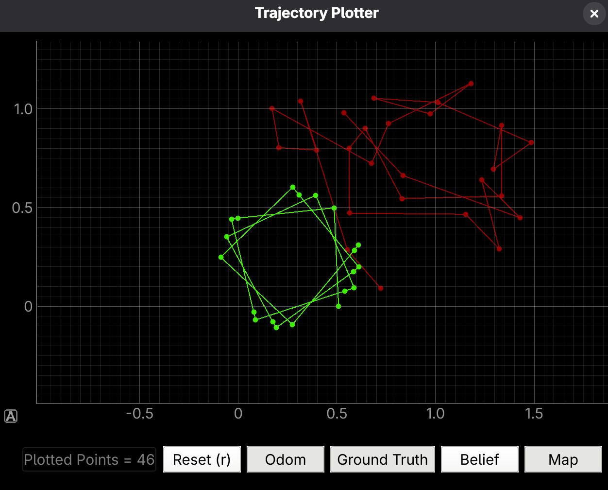
The linear and angular velocity durations are 1 second. In the ground truth, the robot makes a pattern with an overshooting angle. However, the odometry data quickly becomes unpredictable and occupies a much larger state space.
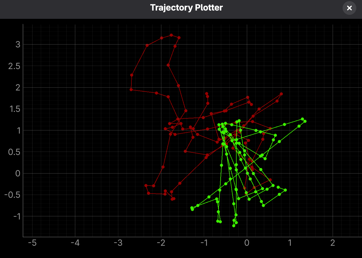
Next, closed loop with simple proportional control was implemented to perform simple obstacle avoidance.
I made the virtual robot turn 90 degrees when close to an obstacle. It slows down proportionally to its distance when it is close to an obstacle (which I defined as 0.8 m). Otherwise, the robot moves at 1 m/s.
Problems with obstacle avoidance included:
- There is no side ToF sensor, so the robot could avoid a front obstacle, but then turn and crash into a side wall. Ideally, there would be multiple side ToF sensors to determine whether to turn left, turn right, or to reverse.
- The car has width, so it could crash into or get stuck on the corner of the square obstacle, though the sensor reads a high distance.
- Experimenting with the gain value and decreasing it makes avoidance more consistent.
cmdr.reset_plotter()
cmdr.reset_sim()

while cmdr.sim_is_running() and cmdr.plotter_is_running():

    tof = cmdr.get_sensor().item()
    Kp = 0.5
    close = 0.8

    if (tof < close):
        cmdr.set_vel(float(Kp*(close-tof)), math.pi)
    elif (tof < 0.1):
        cmdr.set_vel(-1, 0)
    else:
        cmdr.set_vel(1, 0)

    await asyncio.sleep(0.5)

    pose, gt_pose = cmdr.get_pose()

    cmdr.plot_odom(pose[0], pose[1])
    cmdr.plot_gt(gt_pose[0], gt_pose[1])
Grid Localization
Grid localization is performed using Bayes Filter with several Python helper functions.
compute_control(cur_pose, prev_pose) finds the control needed to transition between two poses using geometry. Additionally, the angles are normalized to [-180,+180) degrees from the original [0, 360).
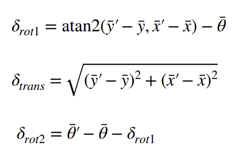
def compute_control(cur_pose, prev_pose):

    delta_rot_1 = mapper.normalize_angle(np.arctan2((cur_pose[1] - prev_pose[1]) , (cur_pose[0] - prev_pose[0])) - prev_pose[2])
    delta_trans = np.hypot(cur_pose[0] - prev_pose[0], cur_pose[1] - prev_pose[1])
    delta_rot_2 = mapper.normalize_angle(cur_pose[2] - prev_pose[2] - delta_rot_1)

    return delta_rot_1, delta_trans, delta_rot_2
Next, the odom_motion_model(cur_pose, prev_pose, u) calculates the actual control using odometry readings. A Gaussian function is used to find the probability the robot can transition given the control action.
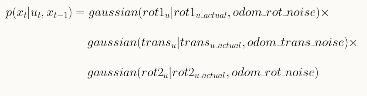
In the localization.py file, the gaussian function is defined as:
    def gaussian(self, x, mu, sigma):
        return np.exp(-np.power(x - mu, 2) / (2*np.power(sigma, 2)))
The gaussian takes in the actual control, the predicted control, and the noise. Then, the total probability p(x'|x, u) is calculated.
def odom_motion_model(cur_pose, prev_pose, u):

    actual_u = compute_control(cur_pose, prev_pose)

    rot1u_actual = actual_u[0]
    transu_actual = actual_u[1]
    rot2u_actual = actual_u[2]

    rot1u = u[0]
    transu = u[1]
    rot2u = u[2]

    p1 = loc.gaussian(rot1u_actual, rot1u, loc.odom_rot_sigma)
    p2 = loc.gaussian(transu_actual, transu, loc.odom_trans_sigma)
    p3 = loc.gaussian(rot2u_actual, rot2u, loc.odom_rot_sigma)

    prob = p1*p2*p3

    return prob
Next, the Bayes Filter consists of a prediction and update step.
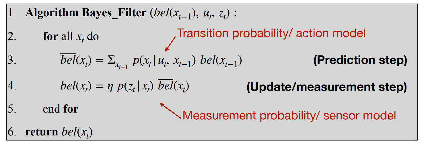
The prediction_step, or the first step of the Bayes Filter, finds the probability for every possible pair of previous and current poses by calling odom_motion_model and mapping the cell to continuous world coordiantes with from_map.
It loops through each cell for both the previous and current poses, where states with a probability < 0.0001 are skipped. The final step sums up the probabilities and stores it in the bel_bar 3D array, which is normalized.
def prediction_step(cur_odom, prev_odom):

    actual_u = compute_control(cur_odom, prev_odom)
    loc.bel_bar = np.zeros((mapper.MAX_CELLS_X, mapper.MAX_CELLS_Y, mapper.MAX_CELLS_A))

    for x1 in range(mapper.MAX_CELLS_X):
        for y1 in range(mapper.MAX_CELLS_Y):
            for a1 in range(mapper.MAX_CELLS_A):
                if (loc.bel[x1,y1,a1] > 0.0001):
                    for x2 in range(mapper.MAX_CELLS_X):
                        for y2 in range(mapper.MAX_CELLS_Y):
                            for a2 in range(mapper.MAX_CELLS_A):
                                p = odom_motion_model(mapper.from_map(cur_odom[0],cur_odom[1],cur_odom[2]),
                                                      mapper.from_map(prev_odom[0],prev_odom[1],prev_odom[2]),
                                                                      actual_u)
                                prior_belief = loc.bel[x1, y1, a1]
                                loc.bel_bar[x2,y2,a2] += p*prior_belief

    loc.bel_bar /= np.sum(loc.bel_bar) # normalization
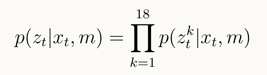
The sensor_model returns an array containing the probabilities of each of the 18 sensor measurements, or p(z|x).
def sensor_model(obs):

    prob_array = np.zeros(18)

    for i in range(18):
        p = loc.gaussian(obs[i], loc.obs_range_data[i], loc.sensor_sigma)

        if isinstance(p, np.ndarray):
            p = p.item()

        prob_array[i] = p

    return prob_array
The final step is the update_step. Each cell is updated on their belief based on p(z|x) and the prediction step belief (bel_bar). The final belief is normalized.
The product of each of the sensor measurements is computed to find the total probability:
def update_step():
    """ Update step of the Bayes Filter.
    Update the probabilities in loc.bel based on loc.bel_bar and the sensor model.
    """
    for x in range(mapper.MAX_CELLS_X):
        for y in range(mapper.MAX_CELLS_Y):
            for a in range(mapper.MAX_CELLS_A):
                loc.bel[x,y,a] = np.prod(sensor_model(mapper.get_views(x,y,a))) * loc.bel_bar[x,y,a]
    loc.bel /= np.sum(loc.bel)
Running the Bayes Filter
Using the above functions, the Bayes Filter is run using a defined trajectory. The robot is initialized with a uniform probability distribution.
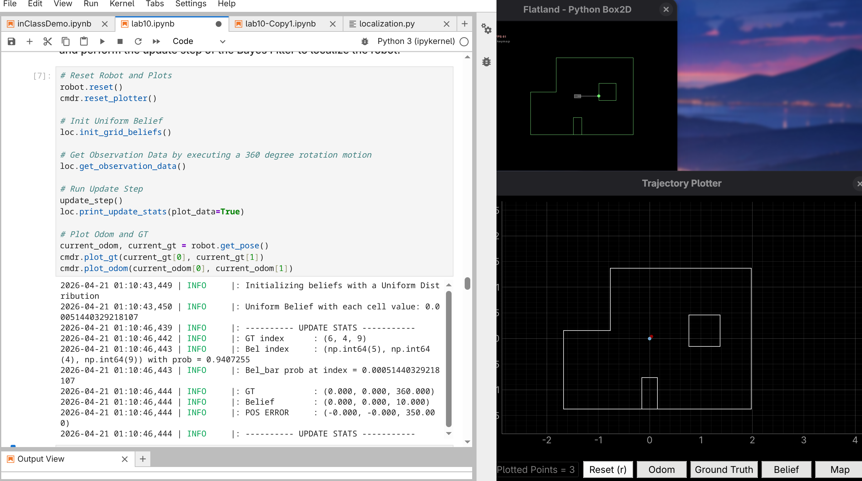
In each iteration, the filter executes the robot's linear motion, performs the prediction step, executes the robot's angular motion to read sensor data, and performs the update step.
The full iteration loop is shown below, displaying the prediction and update information, robot trajectory, odometry readings (red), ground truth (green), and the beliefs (blue).
We observe that the odometry readings quickly become unreliable and stray from the ground truth. In general, the beliefs match with the ground truth. The Bayes Filter performs best when the robot is close to corners or walls due to more accurate sensor data. For example, the narrow hallway on the right side shows less error than in the center.
Collaborations
Stephan's site was referenced for the normalization expression and debugging the prediction + update steps.