Lab 9: Mapping
Building a map of a static room.
Orientation Control
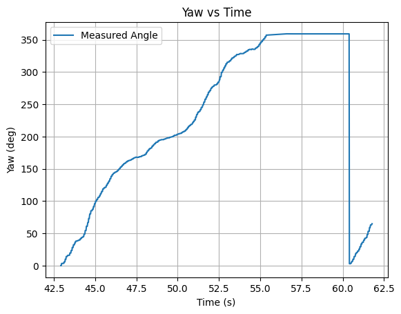
I decided to implement orientation control, where the robot should have at least 14 readings per full rotation. I chose this over angular speed control since the gyroscope DMP measurements are very accurate and the car can do on-axis turns as shown in Lab 7.
First, the angular PID function must be modified to automatically perform incremental turns for a full 360 degrees. Since we need at least 14 measurements, I decided to increment every 20 degrees.
      int increment = 20;
      int angleTraveled;

      if (collectPIDangle) {

        if (!angleInitialized) {
          angleTraveled = 0;
          angleWanted = gyro_yaw + increment; // set first point
          angleInitialized = 1;
        }
        if (angleTraveled < 360){
          pwm = PID_angle_control();
          get_PWM();

          int pwm_max = 255 * Spa;
          int pwm_min = 95;
          abs_pwm = abs(pwm) * pwm_max / 100;
          if (abs(errorCur) < pwm_angle_tolerance) {
            driveState = STOP;
            angleWanted += increment;
            angleTraveled += increment;
          } else {

            if (abs_pwm > pwm_max) abs_pwm = pwm_max;
            if (abs_pwm < pwm_min) abs_pwm = pwm_min;

            if (pwm > 0) driveState = RIGHT;
            else if (pwm < 0) driveState = LEFT;
          }
        } else {
          driveState = STOP;
          collectPIDangle = 0;
        }
      }
Now, when the collectPIDangle flag is set on, the car sets the first wanted angle depending on its current orientation. Then, for a full rotation, it changes its wanted angle in increments of 20 degrees, moving to the next when the tolerance value is reached.
I conducted additional trials to find the turn calibration value so that the car turns evenly about the axis. I implemented a command to change the value over Bluetooth, and the final turn_calibration was 1.15. I also modified the turn gains:
Kpa = 0.06
Kia = 0.002
Kda = 0.08
Spa = 0.6
A trial video is shown below:
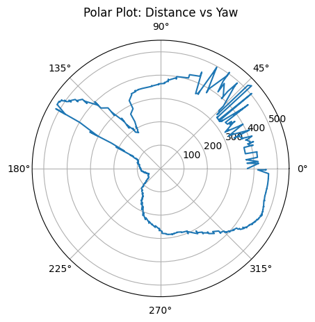
When first converting the data into a polar plot, I noticed that some data would overlap since the car oscillates:
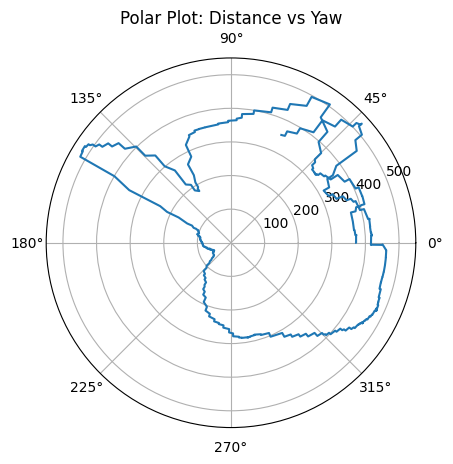
I then sorted the data by the yaw angle, which transforms the overlaps into sharp peaks:
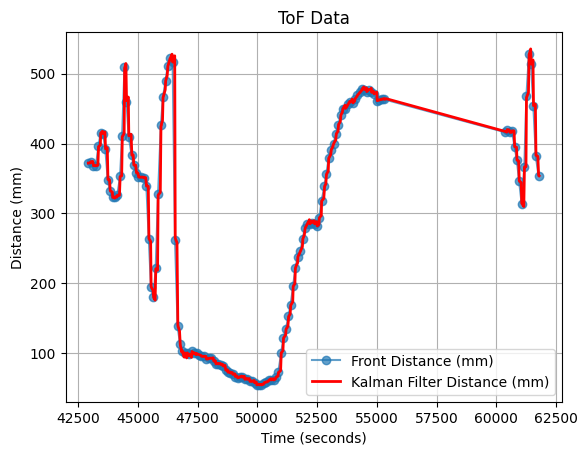
The ToF sensors have an estimated error of +-25mm. The DMP measurements are accurate and its error is negligible. My hardcoded angle tolerance for PID control was 3 degrees. Lastly, drift from the axis is estimated to be 50mm.
Reading Distances
I then executed the data collection at 5 marked locations, making sure to start the robot facing in the top direction for each trial. The end of each trial is signified by the blinking LED.
Note that the PWM values alternate between the minimum value to overcome friction, 95, and 0. I experimented with changing the gain values further to have varied values above 95, but found that the car was likely to spin out of control. I decided it was best to keep close to the minimum PWM values.
(-3, -2)
.png)
.png)
.png)
(5, -3)
.png)
.png)
.png)
(5, 3)
.png)
.png)
.png)
(0, 3)
.png)
.png)
.png)
(0, 0)
.png)
.png)
.png)
Creating Inertial Reference Frame Map
To convert our polar measurements into a cartesian map, we use this transformation matrix (only 2D is required since the car does not rotate or translate in the z direction):
$$ \begin{bmatrix} cos(\theta) & -sin(\theta) \newline sin(\theta) & cos(\theta) \end{bmatrix} $$
In Python, I imported the logged CSV files, matched the yaw angles with the closest time-aligned ToF/Kalman Filter data, and converted the polar data into the inertial reference frame. The marked locations are in feet, which I converted into mm. I also estimated the distance between the front ToF sensor and the center axis of the car to be ~75mm, which I subtracted from the IMU values.
Lastly, since the car started facing towards the top, a 90 degree offset was needed. After doing manual fitting, I determined a 105 degree offset was more accurate to the true map. The reason could be misproper attachment of the sensor leading to an angle skew, or a data buffer.
for file, color in zip(files, colors):
...
    merged = pd.merge_asof(
        merged,
        imu,
        on="time",
        direction="nearest"
    )

    merged = merged.dropna()

    theta = np.deg2rad(merged["yaw"].values.astype(float)) + np.deg2rad(105)
    r = merged["r"].values.astype(float)

    x = (r - tofOffset) * np.cos(theta) + x0*0.3048*1000
    y = (r - tofOffset) * np.sin(theta) + y0*0.3048*1000
...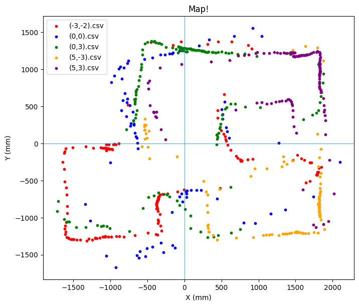
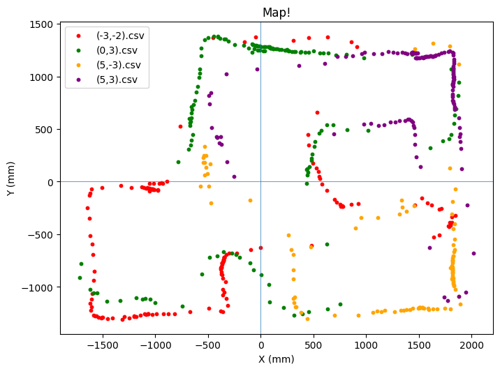
Only the (0,0) point seemed inaccurate after the angle adjustment, which I determined is likely from user error in setting up the trial, starting from an angle as seen in the video.
Therefore, I decided to remove the optional (0,0) data from the map.
Line-Based Map
The last step is to convert the scatter-plot map into a line-based map. I manually estimated the wall boundaries, put the start and end points of each line into lists, and drew them ontop of the current map.
starts = [(-1600, -1300), (-1600, 0), (-800, 0), (-500, 1400), (500, 1200), (1850,1200), (1850, -1200), (350, -1200), (350, -600), (-350, -650), (-350, -1200),
         (600,500), (1400,600), (1500, -200), (700, -200), (500, 200)]
ends = [(-1600,0), (-800, 0), (-500, 1400), (500, 1200), (1850, 1200), (1850, -1200), (350, -1200), (350, -600), (-350, -650), (-350, -1200), (-1600, -1300),
       (1400,600), (1500, -200), (700, -200), (500, 200), (600,500)]

for (x_start, y_start), (x_end, y_end) in zip(starts, ends):
    plt.plot([x_start, x_end], [y_start, y_end], color = 'c', marker='o', linewidth=3)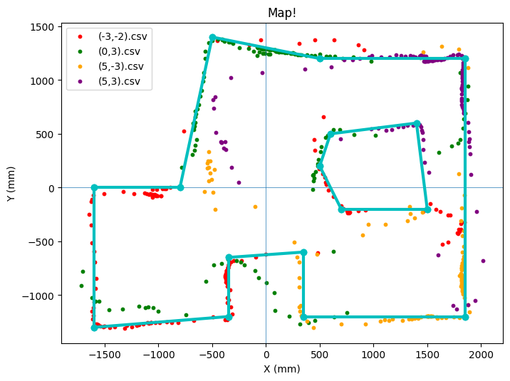
I took some liberties in choosing which data points to consider vs. ignore. I put more trust into points closer to their respective car locations. For example, in the bottom right corner, I mostly based the map off of the yellow points. On the left side, I based the map off of red and green, and ignored yellow.
Overall, the map resembles the true layout, but has errors in the true wall angles, which should all be perpendicular. Additionally, the bottom wall indent is more narrow in the true layout, and the box in the top right was difficult to model accurately.
Utilizing the Kalman Filter data gave more points to work with, but also introduced more noise and inaccurate measurements. Still, it is an improvement over using only the sensor data.
Collaborations
ChatGPT was used for converting to polar plots and setting up the inertial-based map.