Lab 7: Kalman Filter
Implementing a Kalman Filter to replace extrapolated data.
Prelab
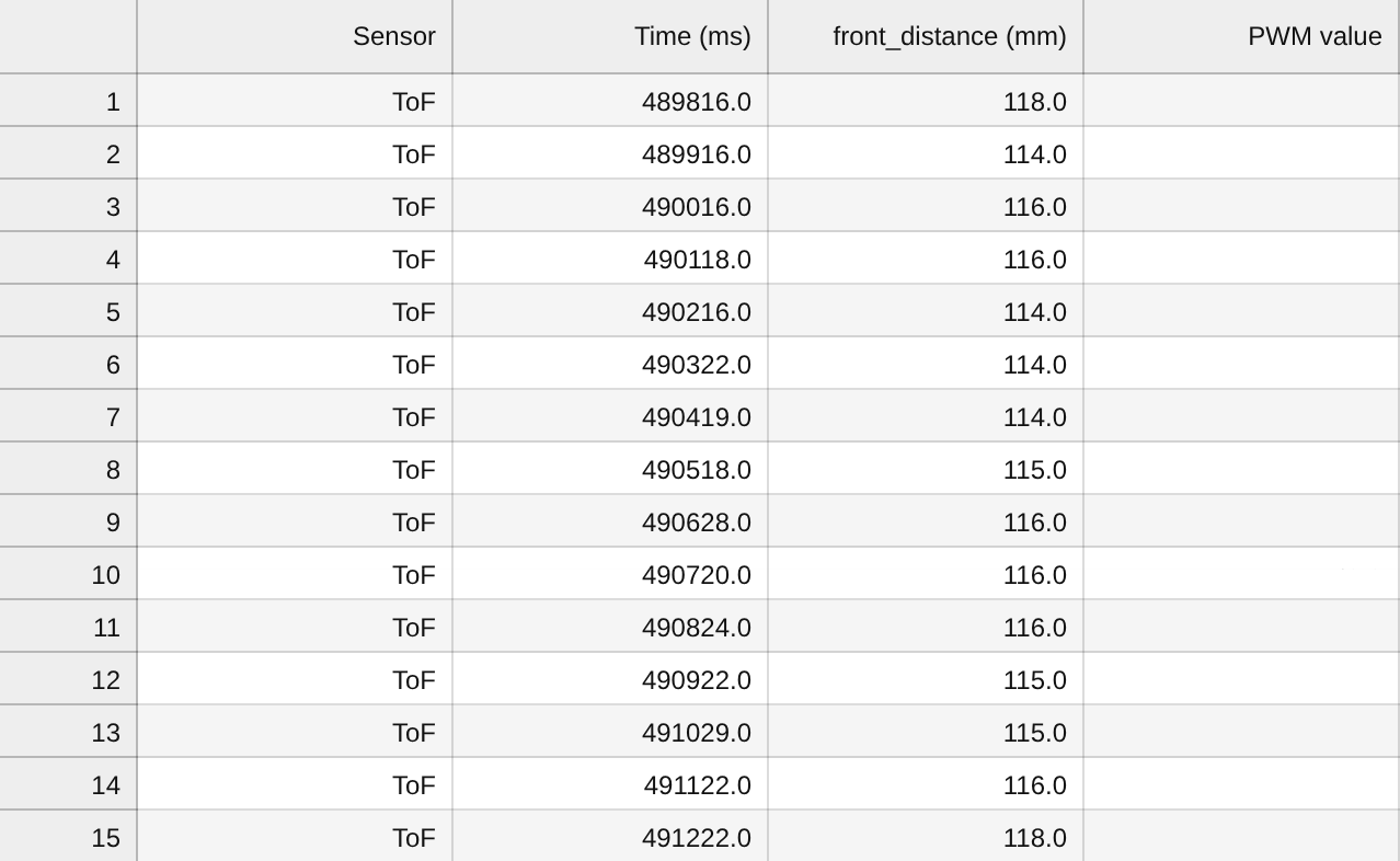
I verified that the ToF sensor and PWM data could be sent over Bluetooth and logged:
I changed the DRIVE command to also take a PWM value, allowing an input of a constant motor speed:
    case DRIVE:
      {
        ...

        int speed;
        success = robot_cmd.get_next_value(speed);
        if (!success) return;

        abs_pwm = speed;

        ...
      }
Lastly, I commented out the extrapolation lines, as it will be replaced by the Kalman Filter values, and I adjusted the collect_tof function to stop the motors and send the data over Bluetooth when set to 0.
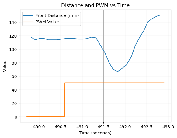
I ensured the system worked by testing with a moving box and measuring the front distance:
Estimating Drag and Momentum
The drag and momentum terms need to be estimated by driving the car towards a wall with a constant step response. Since Lab 5 used 255 for the maximum PWM, I used 50%, rounded up to 128.
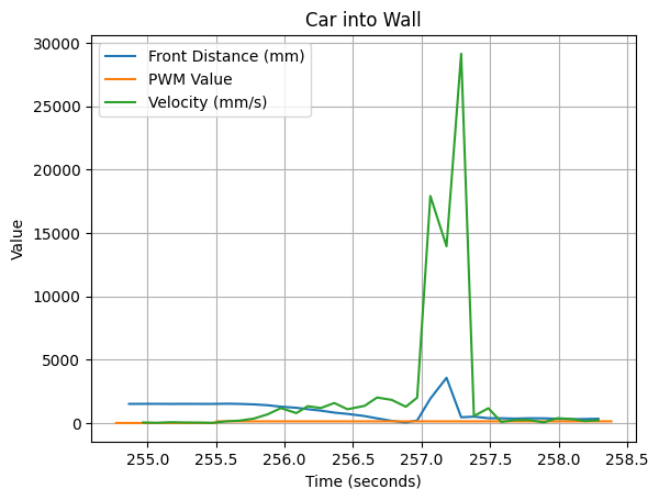
I set up the car as far away from the wall (while remaining within the 2m sensor range) so that it could reach steady state. After crashing into the wall, the sensor data would peak, so I removed the data right after the crash by manually setting the distance threshold. Active braking was already implemented in Lab 6.
The speed was directly calculated from the ToF measurements. The distance, PWM value, and speed were plotted, showing the full data and the data before the crash:
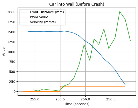
The estimated steady-state speed is 1.75 m/s. The estimated 90% rise time is around 0.8 seconds to reach 1.575 m/s. The u_ss term is 0.5, since we used 50% of the maximum. Now, we can determine the drag and momentum terms:
$$ d = \frac{u_{ss}}{\dot{x}_{ss}} = \frac{0.5}{1.75} ≈ 0.2857 kg/s $$
$$ m = -d * \frac{t_r}{ln(1-d*\dot{x}_{ss})} = -0.2857 * \frac{0.8}{ln(1-0.5)} ≈ 0.33 kg $$
Initializing the Kalman Filter
The A and B matrices and their discretized versions were computed in Python, where n represents the 2 states, and Delta_t is the 30ms sensor timing budget.
d = 0.2857
m = 0.33
n = 2
Delta_t = .03

A = np.array([[0, 1], [0, -d/m]])
B = np.array([[0],[1/m]])

Ad = np.eye(n) + Delta_T * A
Bd = Delta_t * B
The data from the CSV file was extracted, and the crash distance threshold was selected depending on the trial:
df = pd.read_csv("wall1.csv")
tof_df = df[df['Sensor'] == 'ToF']
tof_time = tof_df['Time (ms)'].to_numpy()
tof = tof_df['front_distance (mm)'].to_numpy()

pwm_df = df[df['Sensor'] == 'PWM']
pwm_time = pwm_df['Time (ms)'].to_numpy()
pwm = pwm_df['PWM value'].to_numpy()

crash_threshold = 250
crash_index = np.argmax(tof <= crash_threshold)
Then, the C matrix and state vector were initialized:
C = np.array([[-1,0]])

start = 0
time = time[start:crash_index] - time[start]
tof = tof[start:crash_index]

x = np.array([[-tof[0]], [0]])
Lastly, the process noise and covariance matrices must be determined.
$$ \sigma_1 = \sigma_2 = \sqrt{\frac{10^2}{dt}} $$
$$ \sigma_3 = \sqrt{\frac{10^2}{dx}} $$
Substituting the 30ms ranging time for dt, and an estimated 25mm sensor error, we obtain the values ~58 and ~ 63, which is also used for the initial sigma/noise matrix.
sigma_1 = 58
sigma_2 = sigma_1
sigma_3 = 63

sigma_u=np.array([[sigma_1**2,0],[0,sigma_2**2]])
sigma_z=np.array([[sigma_3**2]])
sigma = np.array([[58**2, 0], [0, 63**2]])
Implementing Kalman Filter (Simulated)
The Kalman Filter is first implemented in Python without the robot.
Since the speed of PWM data is much faster than the ToF readings, I extrapolated the ToF values to match number of PWM values.
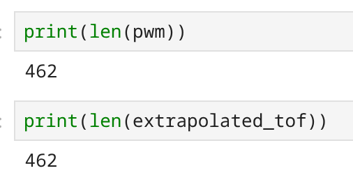
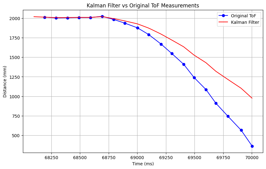
Using the above variances, the Kalman Filter data and the original ToF data is graphed:
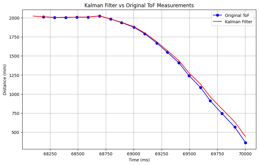
Increasing $\sigma_1$ or $\sigma_2$ represents a decrease in the sampling time dt, and therefore an increase in trust of the sensor data. Below shows a $\sigma_1$ and $\sigma_2$ of 200 and $\sigma_3$ of 63:
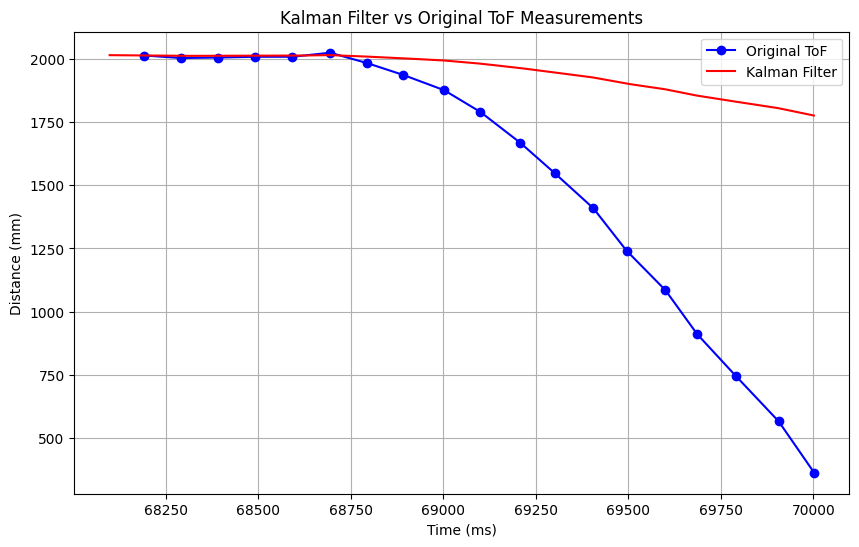
Increasing $\sigma_3$ represents a decrease in the sensor variance dx, and therefore an increase of trust in the model. Below shows a $\sigma_1$ and $\sigma_2$ of 58 and $\sigma_3$ of 200:
I decided on the final values of 80 for $\sigma_1$ and $\sigma_2$, and 25 for $\sigma_3$.

Additional factors that affect the Kalman Filter include:
- The drag and momentum terms, which the A and B matrices build on.
- The sampling time delta_t. An increase in sampling time corresponds to less trust in the sensor data.
- The sampling time of the PWM/PID loop, which affects the extrapolated ToF sampling time in the simulated version.
- THe initial x value, which takes the first ToF sensorvalue in the simulated version, but depends on the ToF sampling time in the live version.
Implementing Kalman Filter (Robot)
Now that the Kalman Filter has been tested on logged data, it can be implemented on the live robot data. kfArray and kf_count were initialized to hold the Kalman Filter values to later compare against the raw data.
The Kalman Filter initialization was rewritten in C++:
Matrix<2,2> Ad = {1, 0.033, 0, 0.971};
Matrix<2,1> Bd = {0, 0.909};

Matrix<1,2> C = {1, 0};
Matrix<2,1> x = {0, 0};

float sigma_1 = 80;
float sigma_2 = sigma_1;
float sigma_3 = 25;

Matrix<1,1> uMatrix = {Sp};

Matrix<2,2> sigma_u = {sigma_1*sigma_1, 0,
                       0, sigma_2*sigma_2};
Matrix<1,1> sigma_z = {sigma_3*sigma_3};

Matrix<2,2> sigma = {58*58, 0,
                    0, 63*63};
In the get_TOF function, the x matrix is initialized to the first ToF value.
  if (tof_count == 0) {
    x = {distanceFront, 0};
  }
Next, the kf function was rewritten in C++, which takes an additional tofReady boolean to check whether to return updated or predicted values:
float kf(Matrix <2,1> &mu, Matrix <2,2> &sigma, Matrix<1,1> u , float y, bool &tofReady){

  int tkf = millis();

  Matrix<2,1> mu_p = Ad * mu + Bd * u;
  Matrix<2,2> sigma_p = (Ad * (sigma * ~Ad)) + sigma_u;

  if (tofReady){ // update
    Matrix<2,2> identity = {1, 0,
                          0, 1};

    Matrix<1,1> sig_m = (C * (sigma_p * ~C)) + sigma_z;
    Matrix<2,1> kkf_gain = sigma_p * (~C * (Inverse(sig_m)));

    Matrix<1,1> y_m = y - (C * mu_p);
    mu = mu_p + kkf_gain * y_m;
    sigma = (identity - (kkf_gain * C)) * sigma_p;
  }
  else { // return prediction
    mu = mu_p;
    sigma = sigma_p;
  }

  tofReady = 0;
  if (kf_count + 1 < maxSize) {
      kfArray[kf_count] = tkf;
      kfArray[kf_count + 1] = mu(0,0);
      kf_count += 2;
  }
  return mu(0,0);
}
Finally, in the main loop, the kf function is called and updates the distanceFront value:
      if (collectTOF && (collectPID || collectPIDangle)) {
        get_PWM();

        if (distanceSensorFront.checkForDataReady() && distanceSensorSide.checkForDataReady()) {
          tofReady = 1;
          get_TOF();
        } else {
          tofReady = 0;
        }
        float kfVal = kf(x, sigma, uMatrix, distanceFront, tofReady);
        distanceFront = kfVal;
      }
In the Jupyter side, I command the robot forward until it reaches the 1 ft distance from the wall, similar to Lab 5 but with a faster PID loop due to the Kalman Filter. I also decided to increase the max PWM speed and retune the gains to improve performance.
Several trials were recorded with varying speeds and gains.
Trial 1:
Kp = 0.1
Ki = 0.002
Kd = 0.25
Sp = 0.8
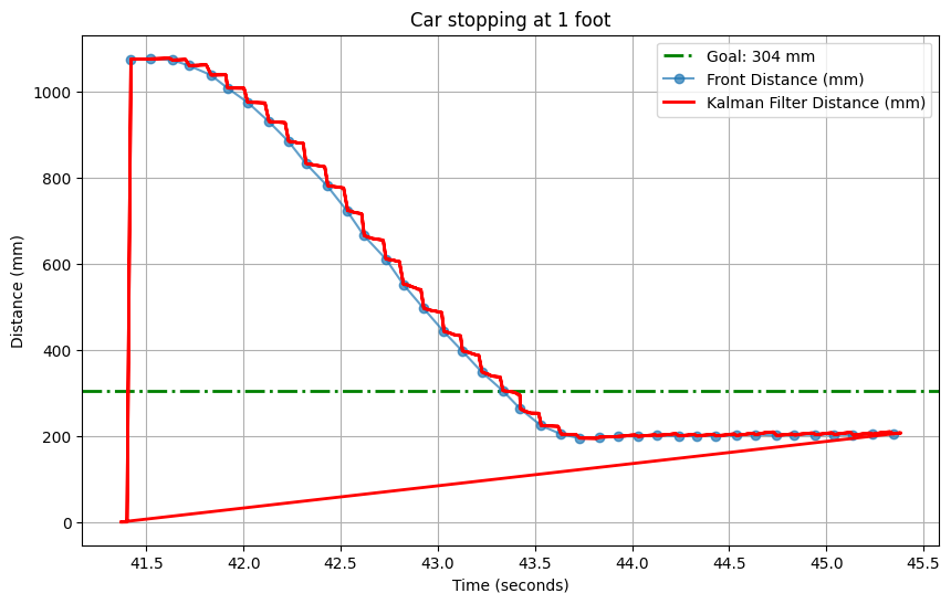
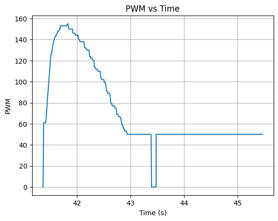
(Note that the straight line in the Kalman Filter is due to an error in extracting data, and only the absolute value of PWM is graphed. The Kalman Filter also always starts near 0 since there is some time between the first ToF value being initialized and the start of the PID control.)
Although the PWM is relatively high, reaching around 150, the car does not stop exactly at the wall and oscillates back.
Trial 2:
Kp = 0.05
Ki = 0.001
Kd = 0.12
Sp = 0.6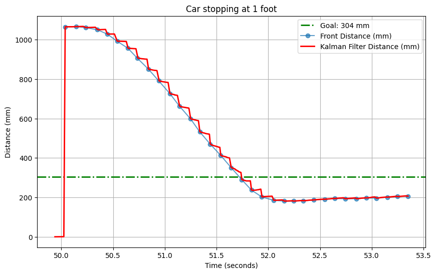
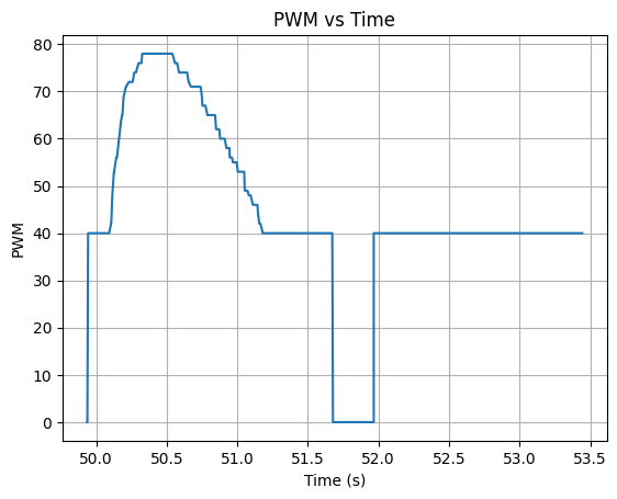
This trial only reaches a max PWM of ~80, but stops without oscillation.
Since the car tends to overshoot the distance goal, improvements could include increasing the deadband range or decreasing the minimum PWM value.
Collaborations
Stephan's site was referenced for comparing plots and sensor variance expressions.
Evan's site was referenced for comparing d and m values, and debugging the Kalman Filter PID control code.
ChatGPT was utilized for the notification handlers, pulling data from the CSVs, extrapolating ToF values, and graphing.