Lab 3: Time of Flight Sensors

2026-02-106 min

Adding the Time-of-Flight (ToF) sensors, wiring and soldering, and testing new ToF and IMU data.

Prelab

The ToF sensor were familiarized with by reading its manual and datasheet. In the technical specifications section, the $I^2C$ is described to have "Up to 400 kHz serial bus programmable address. Default is 0x52."

Since the two ToF sensors have the same hardwired address, we must change one to read all the data. We can either change one of the addresses programmatically or control both through the shutdown (XSHUT) pins. I opted for the programmatic method, since we only need to change the address of the sensor once at power up (by connecting the XSHUT pin to a separate GPIO pin) instead of continuously enabling/disabling the pins.

Next, the placement of the two sensors must be planned. One sensor is placed in the front of the car to detect obstacles the soonest, as it will mostly drive facing forward. The second sensor was placed on the right side so that a wider field of view is covered, and a sensor on the back would be redundant.

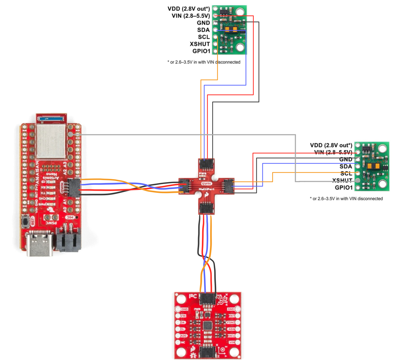
The wiring diagram is shown below, including the ToF sensors, Arduino, and IMU:

Connecting Sensors and Soldering

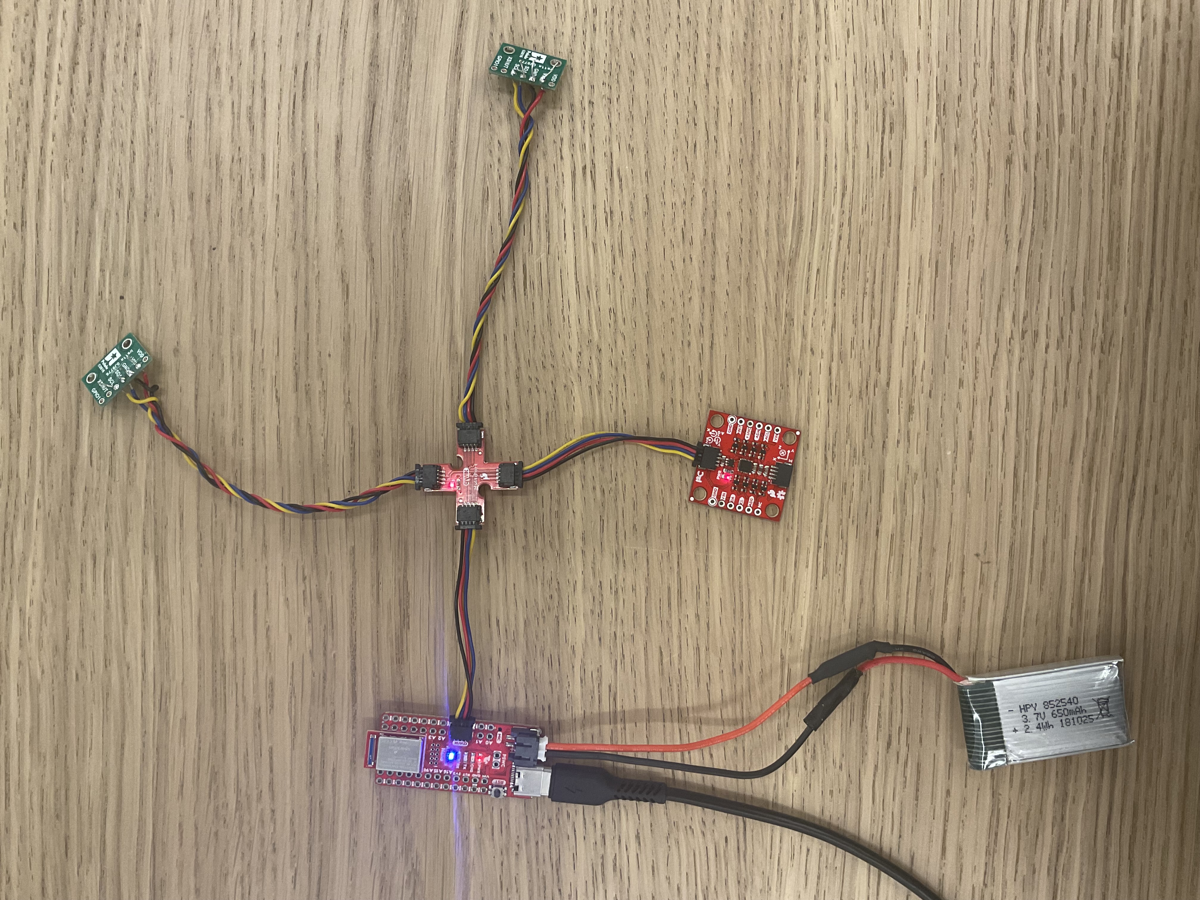
First, the 650mAh battery was wired to the JST jumper wires and the Artemis. The polarity of the JST connector was black to positive and red to negative, so opposite color wires were soldered. The Artemis is now powered using only the battery.

Next, the ToF sensors are soldered to the long QWIIC cables. The VIN, GND, SDA, and SCL pins are soldered to red, black, blue, and yellow respectively.

The Artemis, battery, IMU, and ToF sensors were all connected to the QWIIC break-out board as shown below:

Testing the Sensor Modes

To find the sensor, the Example05_wire_I2C code was run. The address was printed:

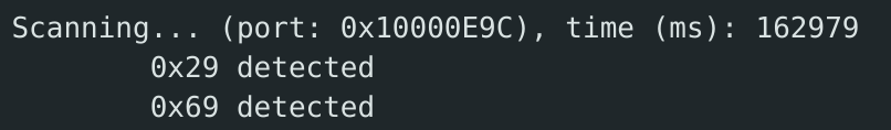
The ToF address is 0x29, and the IMU address is 0x69.

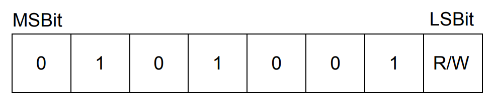
Why does the ToF address not match the expected 0x52? From the datasheet, the 0x52 address is represented by hexadecimal form 01010010. This is read as 0x29, or 00101001, since the last R/W 0 bit is not included.

The sensor modes (short, medium, and long) are optimized based on the maximum expected ranges of 1.3m, 3m, and 4m. Each mode is useful in different scenarios depending on how far we expect our obstacles to be. For example, in a closed-space or a maze, the short mode is useful. Since our robot will be designed to scan the room and maintain position with respect to walls, the long mode is chosen.

The Example1_ReadDistance code was implemented into the main ble_arduino code, where the ToF distances were successfully printed to Serial. Similarly to the IMU collection in Lab 2, a GET_TOF case was written to collect and send sensor data over Bluetooth, and a global collectTOF bool is used to flag the data collection. The main loop checks if the distance sensor is ready:


    case COLLECT_TOF:  
      {

        int collect;

        success = robot_cmd.get_next_value(collect);
        if (!success)
          return;

        if (collect) {
          collectTOF = 1;
          distanceSensorFront.startRanging();
          distanceSensorSide.startRanging();
        
        } else {
          collectTOF = 0;
          distanceSensorFront.stopRanging();
          distanceSensorSide.stopRanging();

        }

        break;
      }

void loop() {

...

  if (collectTOF) {
          if(distanceSensorFront.checkForDataReady() && distanceSensorSide.checkForDataReady()) {
              get_TOF();
            }
  }
}

void get_TOF() {
    float t = millis();

    int distanceFront = distanceSensorFront.getDistance();
    int distanceSide = distanceSensorSide.getDistance();

    tx_estring_value.clear();
    tx_estring_value.append("T:");
    tx_estring_value.append(t);
    tx_estring_value.append("; Front Distance(mm):");
    tx_estring_value.append(distanceFront);
    tx_estring_value.append("; Right Distance(mm):");
    tx_estring_value.append(distanceSide);
    tx_estring_value.append(";");

    tx_characteristic_string.writeValue(tx_estring_value.c_str());
}

First, only one sensor is tested. A notification handler was written to collect arrays of the time, sensor distance, and the manually measured real distance. We take 5 seconds of data points at each "real distance" from a wall, calculate the mean and standard deviation, and plot it.

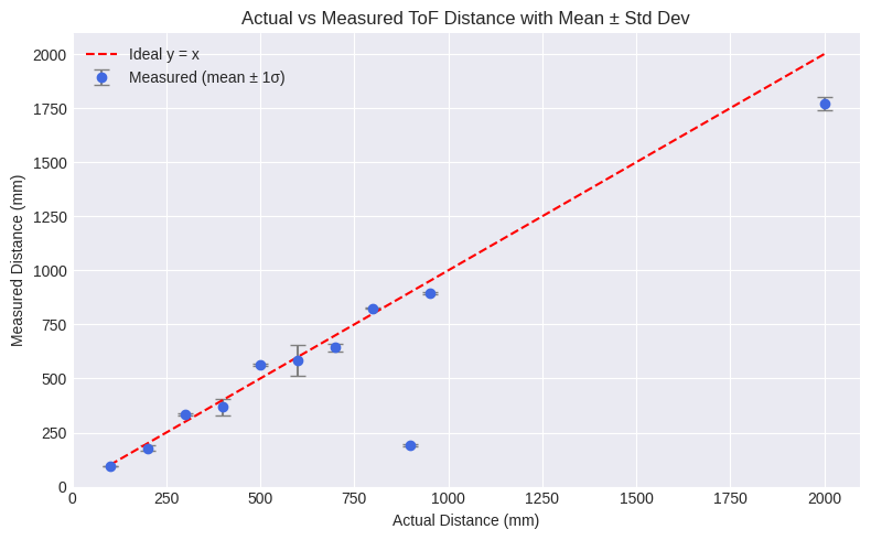
The measurements were taken in around 100mm increments, with 3 seconds of data each. The 900mm measurement is an outlier due to improper testing setup. We can observe that the accuracy unpredictably undershoots or overshoots. However, there are likely errors due to holding the sensor and using a tape measure. The reliability of the sensors is high as the standard deviation values were low.

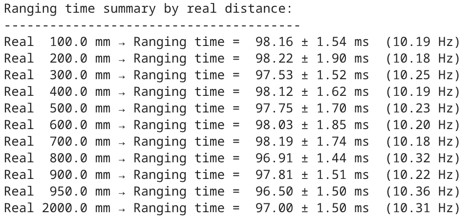
The ranging times for each real distance measure were calculated from the time arrays, which are all around 10 Hz.

Running 2 ToF Sensors

In order to have both ToF sensors working in parallel, the addresses were set to 0x29 and 0x30.

#define XSHUTFRONT 7
#define XSHUTSIDE 8
#define INTERRUPT_PIN 3

SFEVL53L1X distanceSensorFront;
SFEVL53L1X distanceSensorSide(Wire, XSHUTSIDE, INTERRUPT_PIN);

...

pinMode(XSHUTSIDE, OUTPUT); 
pinMode(XSHUTFRONT, OUTPUT); 
digitalWrite(XSHUTSIDE, LOW); 

distanceSensorFront.setI2CAddress(0x29); 

digitalWrite(XSHUTSIDE, HIGH); 
distanceSensorSide.setI2CAddress(0x30);

The data is successfully printed from both sensors:

To test the speed on the sensors in comparison to the main loop, the times are printed to Serial:

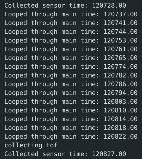
The sensor time matches the above ~10 hz frequency, and the main loop runs at ~250 hz. The get_TOF is only run if both sensors are ready and send the data.

Collecting ToF and IMU Data

Now, we can record both time-stamped IMU and ToF data. A new command is written to set the collectTOF and collectIMU flags.

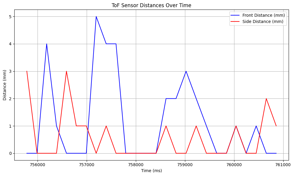
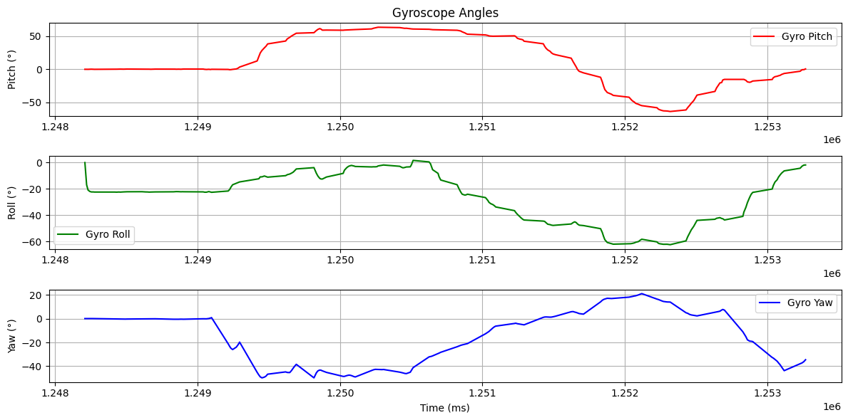
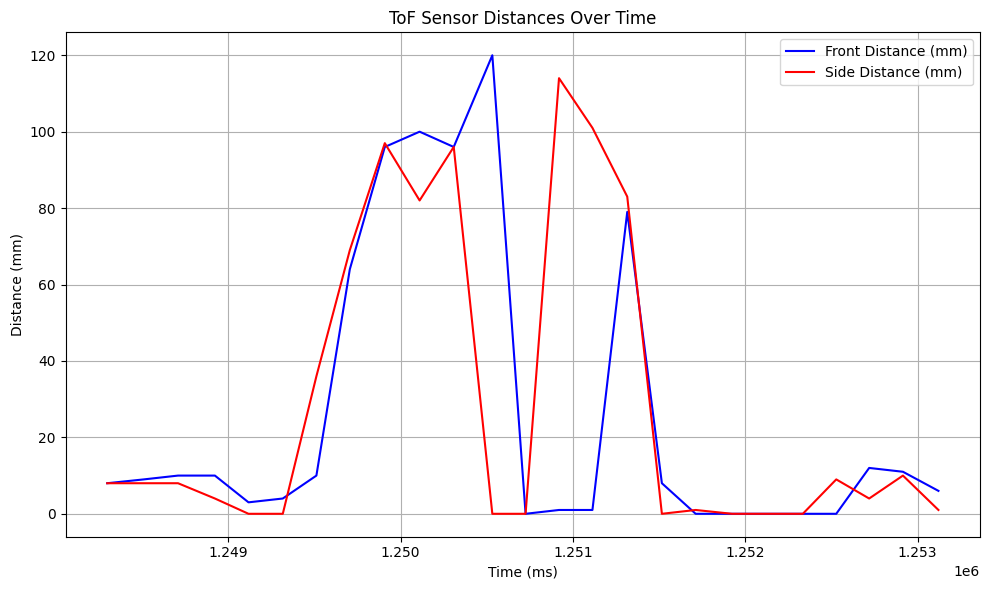
The gyroscope code from Lab 2 was used, with the complementary filter for pitch and roll. Data from both sensors are sent over Bluetooth and plotted over 5 seconds:

Additional Tasks

Infrared Transmission Sensors

ToF sensors (ex. the VL53L1X used in these labs) have multiple distance modes, measuring from 10cm up to 4m, and are mostly insensitive to colors, textures, and lighting. However, they can have repeatability errors due to the low sample rate, and have complicated processing.
Amplitude-based sensors are inexpensive, small, and have a high sample rate. However, they are only used in distances up to 10cm and are sensitive to reflections and lighting.
Triangulation sensors are also mostly insensitive to colors and textures, but not lighting. They are also bulky, have a low sample rate, and have a medium range up to 1m.
LiDaR sensors are the most advanced, mapping in full 3D up to hundreds of meters, but are expensive.

Testing Colors and Textures

To test the effectiveness of the sensors on different materials, the distances were measured at the real distances of 100mm, 200mm, and 300mm. The materials tested were a brown sheet of cardboard, a brown leather notebook cover, a white sheet of paper, and a white sheet of watercolor paper. The results were graphed:

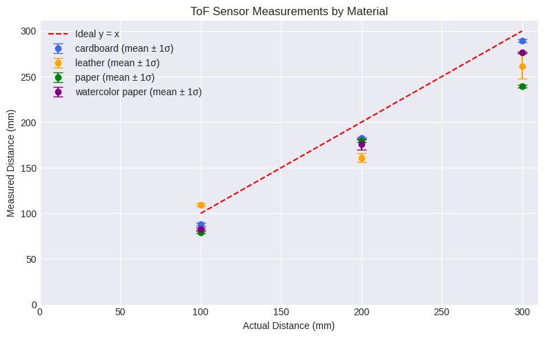
Comparing the brown materials, the cardboard sheet was more accurate than the darker leather. For the white materials, the regular paper was thinner and slightly translucent, so the watercolor paper was more accurate. Overall, the ToF sensors are sensitive to color and texture since it depends on the material's ability to reflect light to calculate the distance and time.

Collaborations

Aidan's page was referenced for the wiring and soldering layout.

Katherine's page was referenced for the prelab start up and $I^2C$ address.

Sensors Lecture Notes were referenced to compare types of infrared sensors.

ChatGPT was used to help graph matplotlib plots, calculate the ranging times, and extract data with the notification handlers.