Lab 2: Inertial Measurement Unit
Adding the IMU, storing data, and setting up the RC car!
Lab 2
Prelab
IMU Setup
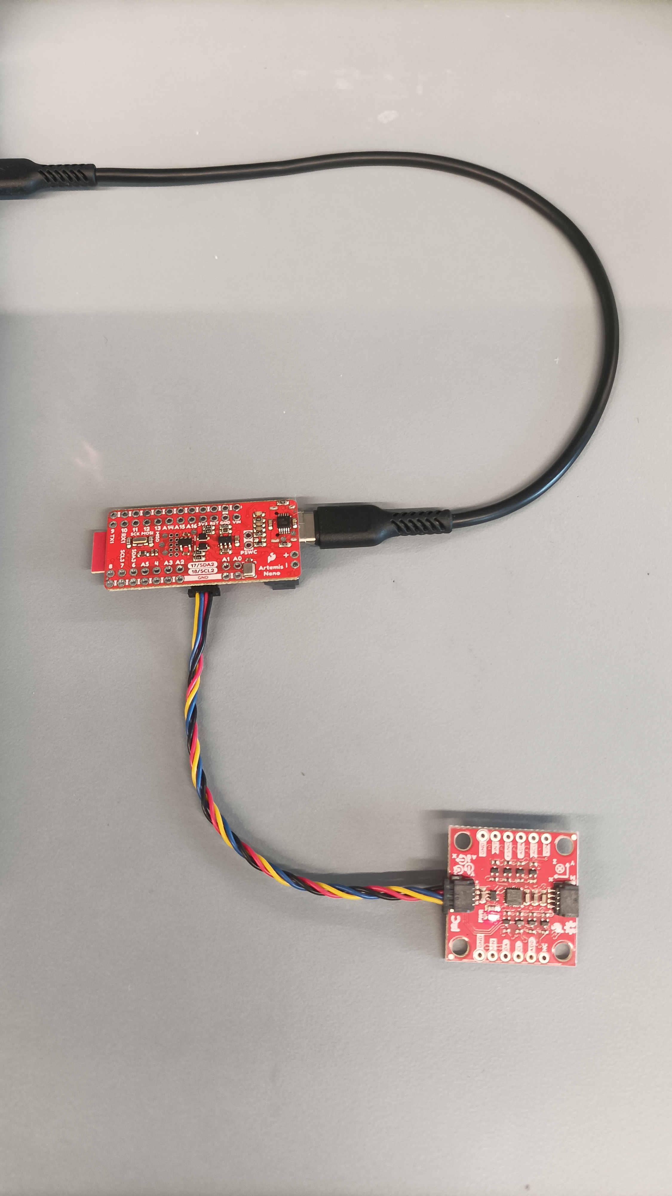
The IMU and Artemis were connected as shown below:
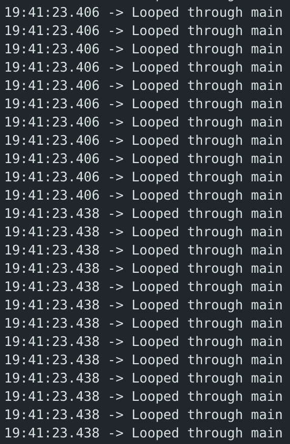
The Example1_Basics code was run, and the IMU data was succcesfully output to the Serial Monitor:
#define AD0_VAL 1This value represents the address of the I2C, as shown in the datasheet, and it was set to 1, the default value. Soldering or closing the ADR jumper would change the value to 0.
The sensor values were read as I accelerated and rotated the board in each axis direction.
The accelerometer values increased when accelerating in the x and y directions. The z value remained constant due to gravity.


Additionally, when the board was flipped, the z direction, gravity, also flipped in value.

The gyrometer values increased when rotating in the x, y, and z directions.


To indicate that the board is running, the Artemis' LED was blinked 3 times in the void setup() function:
  pinMode(LED_BUILTIN, OUTPUT);

  for (int i = 0; i < 2; i++) {

    digitalWrite(LED_BUILTIN, HIGH);
    delay(1000);
    digitalWrite(LED_BUILTIN, LOW);
    delay(1000);

  }
Sampling IMU Data
To start or stop IMU data recording, the COLLECT_IMU case sets the global variable collectIMU to 1 or 0 depending on the sent command.
case COLLECT_IMU:
    {

      int collect;

      success = robot_cmd.get_next_value(collect);
        if (!success)
          return;

      if (collect) {
        collectIMU = 1;
      } else {
        collectIMU = 0;
      }

      break;
    }
The main loop continuously runs the get_IMU() helper function, which checks if the IMU data is ready to be collected, and stores it if so.
if (collectIMU && myICM.dataReady() && (curIMU < (maxSize - 3))) {
      get_IMU();
  }
I decided to store the data in separate arrays for the accelerometer and gyroscope, as it would be easier to parse and analyze the data. Additionally, they are stored as floats since converting the raw data to pitch, roll, and yaw will output decimal values. Although a double would be more precise, it would consume twice as much memory, and the float precision is sufficient for our purposes.
void get_IMU() {
  float t;

    myICM.getAGMT();
    t = millis();
    timeArray[curIMU] = t;
    accArray[curIMU] = (myICM.accX());
    accArray[curIMU+1] = (myICM.accY());
    accArray[curIMU+2] = (myICM.accZ());

    gyroArray[curIMU] = (myICM.gyrX());
    gyroArray[curIMU+1] = (myICM.gyrY());
    gyroArray[curIMU+2] = (myICM.gyrZ());

    tx_estring_value.clear();
    tx_estring_value.append("T:");
    tx_estring_value.append(timeArray[curIMU]);
    tx_estring_value.append("; ");
    tx_estring_value.append("Acc:");
    tx_estring_value.append(accArray[curIMU]);
    tx_estring_value.append(", ");
    tx_estring_value.append(accArray[curIMU+1]);
    tx_estring_value.append(", ");
    tx_estring_value.append(accArray[curIMU+2]);
    tx_estring_value.append("; ");

    tx_estring_value.append("Gyro:");
    tx_estring_value.append(gyroArray[curIMU]);
    tx_estring_value.append(", ");
    tx_estring_value.append(gyroArray[curIMU+1]);
    tx_estring_value.append(", ");
    tx_estring_value.append(gyroArray[curIMU+2]);
    tx_estring_value.append(";");

    tx_characteristic_string.writeValue(tx_estring_value.c_str());

    curIMU += 3;
}
By setting up a simple notification handler that prints the received message, and sending the command to collect data for 5 seconds:
ble.send_command((CMD.COLLECT_IMU), 1)
time.sleep(5)
ble.send_command((CMD.COLLECT_IMU), 0)
The following IMU data is printed:
We observe that the IMU data is produced every ~10 ms. Each loop of data sent contains 7 float values (or 28 bytes), we can store around 12500 values from the 350000 bytes of dynamic memory, or ~125 seconds of data collection.
By running a Serial.print command through the main loop:
We observe that the main loop is run every ~1.3 ms, which is 10x faster than the rate of the IMU.
Accelerometer
After receiving the IMU data over bluetooth, a notification handler is set up to extract the accelerometer data. The following equations from lecture were used to convert accelerometer data into pitch and roll in degrees:
theta = math.atan2(accX, accZ) * 180/math.pi
phi = math.atan2(accY, accZ) * 180/math.pi
To determine the accuracy of the accelerometer, the output at either end of the pitch and roll ranges is determined. A flat edge was used to ensure perfect angles.
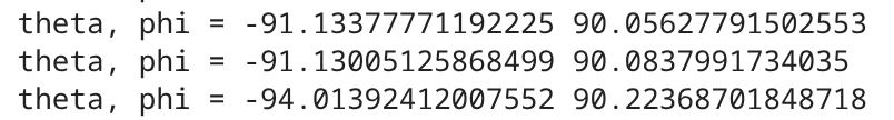
The individual output of the pitch and roll at 90 and -90 degrees is shown:
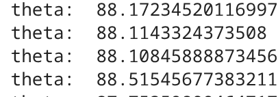
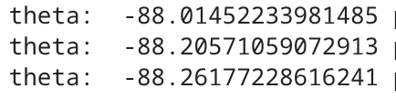
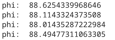
With a two-point calibration, we calculate the conversion factor to be 90/88.2 or ~1.02. The completed notification handler is shown below:
def notification_handler(uuid, byte_array):
m = ble.bytearray_to_string(byte_array)
extract = m.strip().split(';')
time = extract[0].split(':')[1]
acc_values = extract[1].split(':')[1].split(',')
accX, accY, accZ = [float(v.strip()) for v in acc_values]
theta = math.atan2(accX, accZ) * 180/math.pi
phi = math.atan2(accY, accZ) * 180/math.pi
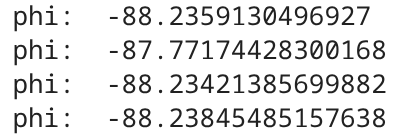
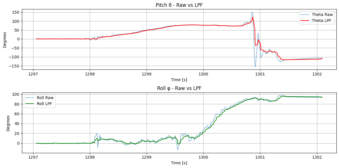
print("theta: ", theta*conversion, "phi: ", phi*conversion)The output of moving the IMU -90 degrees in pitch and 90 degrees in roll is shown:
Next, we analyze the noise produced by the accelerometer data and perform a Fourier Transform. First, the IMU data lying flat on the table is graphed:
Then, a Fourier transform is applied and the results are graphed:
N = int(wait * sample_rate)

theta = np.array(theta_list)
t = np.array(times)

freq_data = fft(theta_list)
y = 2/N * np.abs (freq_data [0:int (N/2)])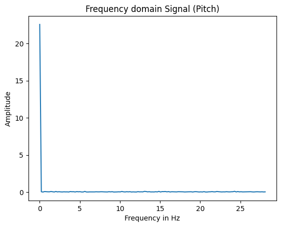
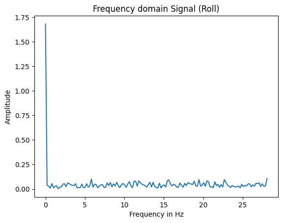
From observation, the cutoff frequency $f_c$ is picked to be 3 hz to mitigate the beginning peaks. A too high cutoff frequency reduces more noise, but may block out wanted signals in which the car experiences sharp changes in angle or turns. To apply a low pass filter, the $\alpha$ value is calculated from the equations, where T represents the inverse of the sampling rate:
$$ \alpha = \frac{T + RC}{T} $$
$$ f_c = \frac{1}{2\pi RC} $$
$\alpha$ is found to be 0.2498.
The new low pass filter values are calculated and graphed:
theta_lpf = np.zeros_like(theta_raw)
phi_lpf   = np.zeros_like(phi_raw)

theta_lpf[0] = theta_raw[0]
phi_lpf[0]   = phi_raw[0]

for n in range(1, len(theta_raw)):
    theta_lpf[n] = alpha * theta_raw[n] + (1 - alpha) * theta_lpf[n-1]
    phi_lpf[n]   = alpha * phi_raw[n]   + (1 - alpha) * phi_lpf[n-1]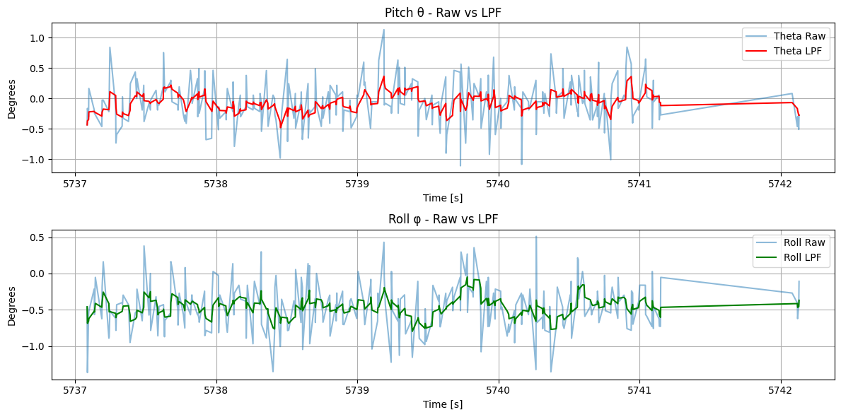
The low pass filter drastically reduces the noise in the pitch and roll values.
Gyroscope
Next, the pitch, roll, and yaw angles are computed from the gyroscope data. We use the following equation from lecture to loop through and plot the data (note that the accelerometer-defined pitch, roll, and yaw correspond to the negative of the gyro's roll, yaw, and pitch):
$$ \theta_g = \theta_g + gyro\_reading*dt $$
for n in range(1, len(gyroX_raw)):
    dt = time_sec[n] - time_sec[n-1]
    gyro_pitch[n] = gyro_pitch[n-1] - gyroY_raw[n]*dt
    gyro_roll[n] = gyro_roll[n-1] - gyroZ_raw[n]*dt
    gyro_yaw[n] = gyro_yaw[n-1] - gyroX_raw[n]*dt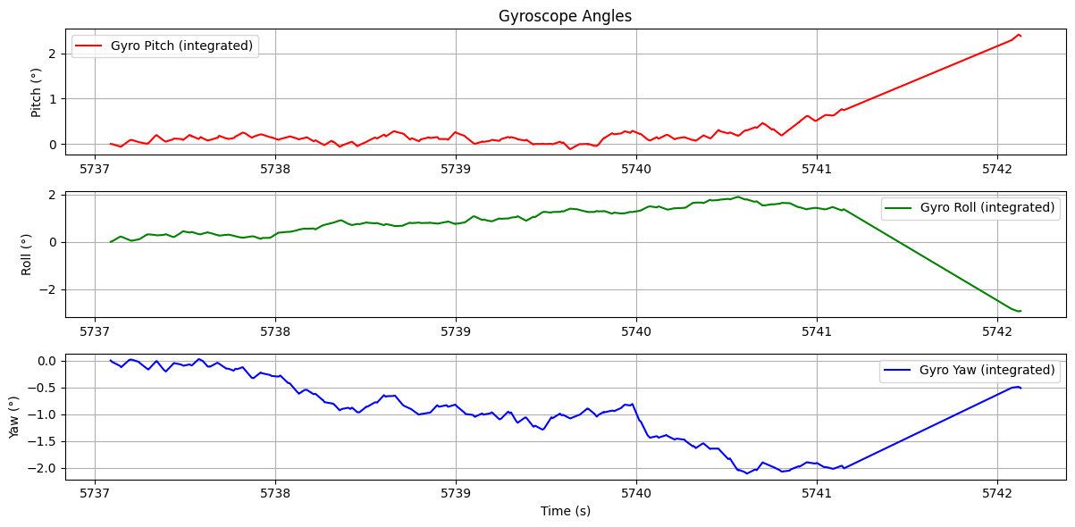
We also plot the data when tilting the IMU:
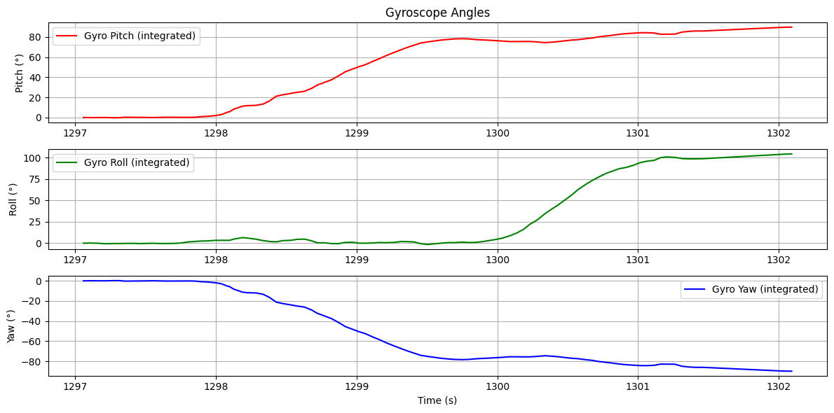
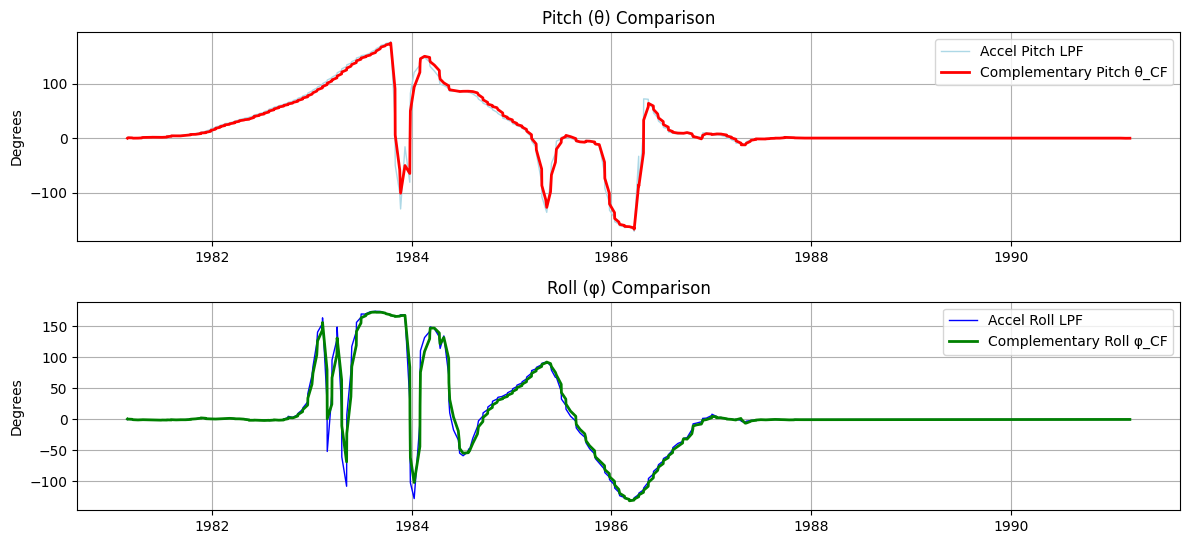
Comparing the gyroscope angles to the above low pass filter graph, we observe that there is lower noise, but the readings began to drift after a few seconds. Therefore, we apply a complementary filter and compare it to the accelerometer's low pass filter:
$$ \theta = (\theta + \theta_g)(1-\alpha) + \theta_a\alpha $$
for n in range(1, len(gyroX_raw)):
    cgyro_pitch[n] = (cgyro_pitch[n-1] + gyroY_raw[n]*dt)*alpha + theta_lpf[n]*(1-alpha)
    cgyro_roll[n]  = (cgyro_roll[n-1]  + gyroZ_raw[n]*dt)*alpha + phi_lpf[n]*(1-alpha)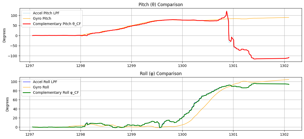
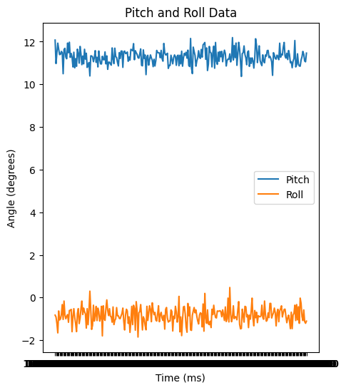
We observe that the low pass and complementary filter data largely overlap each other, and are therefore accurate measurements. The gyroscope's complementary filter is also more stable than the accelerometer's low pass filter.
10 seconds of data were also recorded to demonstrate the range and stability:
RC Car
Lastly, the RC car was remote controlled and observed.
We see that the car is extremely sensitive to controls and is difficult to turn precisely, where even one tap on the remote control makes it turn 90 degrees. It accelerates quickly to max translational and rotational speed, and it easily flips over when running into an obstacle (the wall).
Collaborations
Lucca's page was referenced in how to sample the accelerometer and gyroscope data. Katherine's page was referenced in debugging the complementary filter and comparing graph outputs. ChatGPT was used to help write code for the notification handler, extracting the data, and plotting the graphs. This page was referenced to help plot the Fourier transforms.